Dynamic Range in Excel

Hi reader,

Dynamic ranges are quite useful when you  are using Pivot Tables. They automatically adjust the table range while you insert data a table. Consider the example bellow to understand how to do it.

Method 1 ("Table" option):

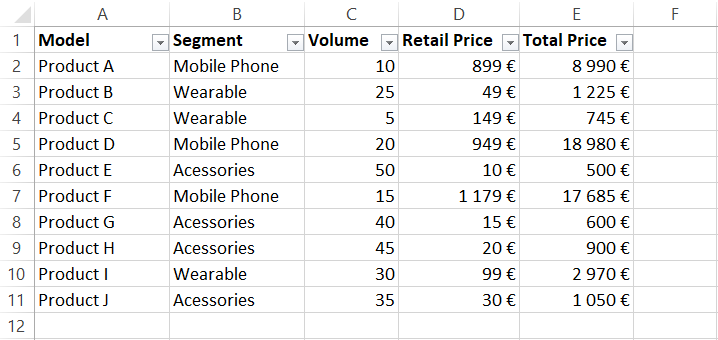
1. Select the table range you want (e.g. range "A1:E11")
2. Click on "Insert" tab and then select "Table"
   
3. Confirm if the range is correct and press "ok" button
   
4. Range had turned dynamic, named by default as "Table1". If you want you can change the name on the "Table Name" box
   
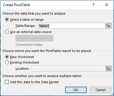
5. Now, just create a "PivotTable", where "Table/Range" is the same as defined in the previous points (e.g. "Table1")
   

Method 2 (offset formula):

1. Click on "Formulas" tab and select "Name Manager" 
   
2. Select “New”, and give a name to the dynamic table (e.g. “Table2”). Then, on “Refers to” use the formula "=OFFSET(Reference;0;0;Height;Width)", where:

• Reference: upper left cell of the table (e.g. cell “A1”)
• Height: number of rows on the table. You can get it automatically by counting the number of rows, on a column that is always fulfilled (e.g. “COUNTA(A:A)”)
• Width: number of columns on the table. You can get it automatically by counting the table header row (e.g. “COUNTA(1:1)”)
  

Now, just insert more information on the table.

Hope it makes your spreadsheets easier.